Zero inflation in ecology

The April Eco-Stats Lab (Friday 24th, 2pm, Bioscience level 6) will be on zero inflated data in ecology. 

It's very common for ecological data to contain many zeros. To account for this we may need to:

1. Use zero inflated regression models

2. Do absolutely nothing (i.e. fit standard glm's)

In this lab we'll talk about why many zeros may occur in ecology, and the appropriate ways to account for them in your analysis.We will mostly use the pscl package in R.

Many Zeros in Ecology

Your abundance data may look like this.

We can see these data have a lot of zeros, and may be zero inflated. Some possible reasons are

1. There is one process (ecological variables like climate etc) governing both presence and abundance. (E.g. species is not abundant in wet whether, and wet whether is common in the dataset)

2. There are two (possibly related) processes, one governing presence, the other abundance (E.g. species can only occur in temperatures above 20°, beyond this abundance is affected by rainfall and time of day)

Do you need zero inflated models for your data with many zeros?

Some of the reasons above require zero inflated models to be fit, but reason 1 does not, and may be a very common reason for excess zeros, see Warton (2005).

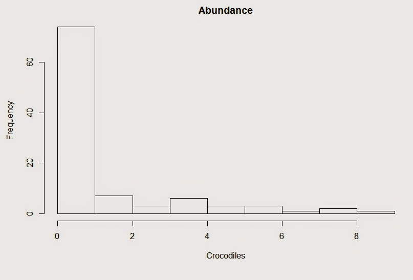
Let's have a look at a simulated example. I have simulated count data which is exactly Poisson distributed, with no zero inflation, but with a mean that depends on temperature though this formula. 

λ = exp( 12.4 -4*log(temp) )

The histogram above is of this dataset I simulated. There are lots of zeros, but I specifically did not simulate a zero inflated model, just a regular Poisson model with an explanatory variable. If I look at the raw counts in isolation, using a histogram, or by applying a test of zero inflation, we would conclude the data is zero inflated, and we would be wrong.

Let’s go to R and fit some models, and see what models fit best.

Download data here. We will use a package called pscl to fit the zero inflated models.

load("Crocs")

library(pscl)

glm.pois=glm(Croc~log(temp),family=poisson,data=Crocs)

zi.pois=zeroinfl(Croc~log(temp) ,data=Crocs) 

AIC(glm.pois,zi.pois)

So AIC is lower for the model with no zero inflation, as expected, since that is the model we simulated from. We can also look at how many zeros are expected by each of these models, and how many we have. This is just to convince ourselves we have a sensible model, it’s not a formal test of anything.

round(c("Obs" = sum(Crocs$Croc < 1),

        "glm.pois" = sum(dpois(0, fitted(glm.pois))),

        "zi.pois" = sum(predict(zi.pois, type = "prob")[,1])))

Note on AIC

The AIC is approximate in this setting, and it may favour the more complex model (in this case the zero inflated model) in some cases where a glm is the better model, but there’s not much harm in that. There are alternatives, like the Vuong test (vuong() in pscl) which may work better, or you could try bootstrap if you’re feeling adventurous.

The Moral of this simulation

Just because your data contains lots of zeros, does not mean its zero inflated. You should fit models with explanatory variables with and without zero inflation, and check which model fits best, using model selection methods (e.g. AIC)

Three complications to zero inflated models

1. Overdispersion

Ecological data is commonly overdisprsed (the variance is larger than the mean). We often address this by using a negative binomial distribution to model data instead of a Poisson distribution. If you believe you have both zero inflation and overdispersion, there is an option in pscl to use a zero inflated negative binomial distribution, This might be a better choice than the zero inflated Poisson, although you can also use AIC to see which fits best. To use the negative binomial distribution add dist="negbin" inside the zeroinfl()function.

2. Hurdle models vs zero inflated models

There are actually two generic ways to model zero inflation, and they differ in terms of whether they attribute some of the zeros to the Poisson (negative binomial) distribution, or whether all the zeros are attributed to a presence/absence process. The zeroinfl() function is the former type, but you can also try the latter type using the hurdle() function instead of the zeroinfl(). They tend to give pretty similar results, and you can test which one is better with AIC. The hurdle models are a little easier to interpret.

3. Same or different explanatory variables for presence/absence and counts.

As mentioned above, there are different reasons for zero inflation. Explanatory variables might only affect counts, or they may affect both counts and presence/absence, or different explanatory variables can affect counts than affect presence/absence. We can fit zero inflated models with all these scenarios by modifying the formula inside the hurdle()or zeroinfl() function. The general formula is

Counts ~ count covariates | presence covariates

e.g. Croc ~ log(temp) | pres

Putting it all together (1+2+3)

hurdle.nb=hurdle(Croc ~ log(temp) | pres , dist="negbin",data=Crocs)

Real data examples

Example 1: Odontophora in tasmania

library(MASS)
library(mvabund)

data(Tasmania)

tas=list(Abund=Tasmania$abund[,47],Trt=Tasmania$treatment)

tas$Abund

glm.nbin=glm.nb(Abund~Trt,data=tas)

hurdle.nbin=hurdle(Abund~Trt|Trt,dist="negbin",data=tas)

zi.nbin=zeroinfl(Abund~Trt|Trt,dist="negbin",data=tas)

AIC(glm.nbin,hurdle.nbin,zi.nbin)

#seems like the glm fits best

#refit with mvabund for better residual plot

glm.nbin=manyglm(Abund~Trt,data=tas)

plot(glm.nbin)

Example 2 – Published papers

data(bioChemists)

chem.glm <- glm(art ~ ., data = bioChemists, family = poisson)

chem.zip <- zeroinfl(art ~ . | ., data = bioChemists)

chem.hurd <- hurdle(art ~ . | ., data = bioChemists)

   

AIC(chem.glm, chem.zip,chem.hurd)

vuong(chem.glm, chem.zip) #can only compare two models

#zero inflated and hurdle models are better for these data

summary(chem.zip)

Extensions

Zero inflated Mixed models

Look at glmmADMB and MCMCglmm for possible implementations, but these are not straight forward to implement. 

Multivariate zero inflated models

MCMCglmm can do multivariate also.

Bibliography

Zuur, Alain, et al. Mixed effects models and extensions in ecology with R. Springer Science & Business Media, 2009.

Warton, David I. "Many zeros does not mean zero inflation: comparing the goodness‐of‐fit of parametric models to multivariate abundance data."Environmetrics 16.3 (2005): 275-289.

Martin, Tara G., et al. "Zero tolerance ecology: improving ecological inference by modelling the source of zero observations." Ecology Letters 8.11 (2005): 1235-1246.

Zeileis, Achim, Christian Kleiber, and Simon Jackman. "Regression models for count data in R." (2007).