Introduction to Docker
It’s become increasingly important to be able to experiment, reproduce workflows and results, share code and to be able to take advantage of large scale data analysis.
Docker is a lightweight virtual machine technology that provides an isolated, self-contained, versioned and shareable linux-based environment that is now the tool of choice in industry. With the growth of cloud computing companies regularly spin up clusters containing hundreds or even thousands of docker instances - and with that there’s been a concurrent growth in management and orchestration tools in the docker ecosystem.
Ok - that’s great - but why should statisticians care?
Because this is a great way to easily scale and share your research while it’s in progress. You can package up work-in-progress R code and data without having to build R packages first.
It also allows you to experiment and test without concerns - for example R 4.0 is now available. Given the choice between testing your work against new versions of R and upgrading your base R installation, an easy solution is to use a Docker container configured with R 4.0 and leave your host machine alone.
Here’s some motivating examples:
Ship & Share - docker promotes reproducibility in research. No matter what needs to be installed in the environment to reproduce your results, you can build a complete machine image packaging up code and data and simply share the image. This is the virtual equivalent of “here - just use my computer. It works on that…”
Docker doesn’t replace the value of building and sharing R packages themselves. The point is simply that you do not have to wait until all your code is packaged any longer and can experiment and collaborate freely while research is in progress.
Basic Concepts
DockerHub - (https://hub.docker.com/) this is the equivalent of GitHub but much coarser. It’s the central repository for versioned Docker images - you can pull images from public repositories for your own use or pull/push images to your own private repositories.
To use Docker you need to signup a free account which automatically gives you access to your own private repositories. There are also enterprise tiers with additional benefits.
Docker Image - this is a blueprint for the machine itself. You can choose from thousands of pre-configured images available at DockerHub, use them as is or as a baseline to customise your own. An image is like a class in programming - it’s used to create instances of the running machine - known as containers.
An image contains all the code, packages and programming environment needed to support the work you want to do. It also has a version associated with it - called a tag.
Docker File - used to build an image. This is where you can specify additional packages, copy source code or add additional linux command line tools to be included in the image. You only need to work with this if you want to customise an image for your own use.
Docker Container - this is a running instance of a machine created from an image. A container is like an object instance created from a programming class. The Docker service on your local machine will instantiate the container for you - you can then connect to it and get busy.
General Notes
While Docker is a mature technology it does have some drawbacks. Docker images are generally a few gigabytes in size and so can quickly take up a lot of space on a standard laptop.
Consequently, pushing and pulling images to and from DockerHub can be time consuming unless you have a fast internet link. This isn’t a big problem as most of the time you’re probably only working with one container image but it’s worth keeping in mind.
Secondly, interfacing with Docker can be daunting. Bare in mind that it was designed by hardcore sys-admin types so there are options (i.e command line switches) for almost anything you can think of.
However there are generally only a few commands to know that will cover almost all use cases which we’ll summarise next.
Docker Command Cheatsheet
These commands are run in a terminal window on your Windows/Mac/Linux host machine:
Login to DockerHub from your host machine:
docker login
This will prompt your for the username and password you used to sign up with DockerHub.
Pull an Image to your local machine:
docker pull rocker/geospatial
This pulls the latest version of the rocker/geospatial image. You can also specify a particular version you want to use by including a tag:
docker pull rocker/geospatial:4.0.2
List images:
docker images
Displays all images you have available on your host:

Launch a container (simple version):
docker run -it chenobyte/geospatial:1.4 /bin/bash
This creates a container using the chenobyte/geospatial:1.4 local image, connects to it and runs a bash shell inside the container. The -it switches ensure the container stays interactive. As can be seen below we are inside the container as root:

Once inside, you can kill or exit the container either by Ctrl+D or by typing exit. This drops you back out to the host terminal. You can also exit back to the host without killing the container by typing Ctrl+PQ. This is known as detaching.
List containers:
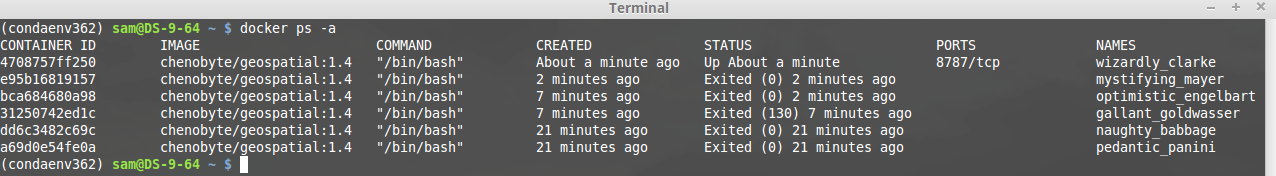
docker ps -a
Displays all containers including their status. Note that docker automatically assigns names to each instance - although you can override this if you really want to:
Attaching to a Running Container:
As seen above, each container has a container identifier. You can attach (jump back into) a running container using the container id:
docker attach <container_id>

Commit a Running Container:
This is useful when you’ve launched a container, made some changes while inside it (say installed some utilities or software) and now want to save the complete container state as a new image that you can reuse later.
The general format is:
docker commit <container_id> name:tag
As an example, if I’ve launched a container using image chenobyte/geospatial:1.5 and then make some changes I want to keep (e.g installed git) , I can detach and save the current container state as a new image. If the container id is 1234 then I can make a new version:
docker commit 1234 chenobyte/geospatial:1.5
I now have a new image version which is just like any other image and can be used to launch new containers too.
Stopping a Running Container:
You stop a running container from the host using the container id:
docker stop <container_id>
Launch a container (complicated version):
docker run -it
-p 8888:8888 \
-v /home/ec2-user/data:/data \
-e NB_UID=$(id -u) \
-e NB_GID=$(id -g) \
-e GRANT_SUDO=yes \
-e GEN_CERT=yes \
--user root \
chenobyte/geospatial:1.4 \
/bin/bash
This example looks daunting but is actually the most useful common case. The main issues are around making sure you have permissions inside the container to write to host directories etc. You don’t need to understand all the -e options - you can just re-use as is.
The -p switch exposes port 8888 inside the container as port 8888 to the host. This is useful when the container is running a server (RStudio, Jupyter etc). See the aside below for more information.
The -v option is probably the most useful. This a volume mapping which says that the directory /home/ec2-user/data on the host should be made available inside the container at /data. In this way, data files or code on the host can be accessed from within the container itself. You can have as many mappings as you want here.
There are many many more available options for running containers including specifying available CPUs and RAM, container lifecycle etc. For more information check out the references in the resources section below.

Building Your Own Image
Docker images are built using a plain text file known as the DockerFile. There are a wide range of options available (see resources below) but the main thing for us is to see how we can use an existing base image, and specify some additional R packages to be installed.
The first line in a Docker file specifies the base image you want to use. For example you might want to use a base image that contains a Shiny server. In that case, (once you’ve found the image on DockerHub) you specify it in the DockerFile:
FROM rocker/shiny:4.0.0
Note - while you don’t have to specify the tag (version) it’s best practice to do so - if you don’t it will use the latest version - which can be updated without you knowing!
You can also specify code to be copied into the image, set the initial working directory, environmental variables and execute commands. In the example below we use the geo-spatial image as the base and install additional R packages.
Note that the process shown below in the RUN command is specific to these R images - these ensure that R packages and dependencies are always installed from a fixed snapshot of CRAN at a specific date.

Once you’ve defined your docker file you create the image and give it a tag. This needs to be run from the same directory as the docker file (note the trailing full stop!). Here we’re saying that the new version of the image is to be tagged as version 1.5:
docker build --tag chenobyte/geospatial:1.5 .
Now your image is built you can create containers with it and push the image back to your repository in DockerHub. This is the bit that can take a while as it’s usually a multi-gigabyte upload:
docker push chenobyte/geospatial:1.5
And now you can share your work with colleagues as an entire self-contained unit.
Summary
This is just a quick introduction but while Docker has a steep initial learning curve, it’s one that’s worth investing the time in. You don’t need to become an expert to take advantage of massive scale compute power either.
Imagine you had a high performance 10-node cluster that you wanted to run a simulation on. You would have to make sure every node had the same R environment, packages, versions and data. By creating a Docker image it doesn’t matter if it’s a 10-node or 100-node cluster. You only need to specify a run time environment once.
In our recent work we used Docker containers across a 4 x 64 CPU node cluster - this allowed us to fit 17 complete large scale spatial models in parallel while using the best allocation of available cluster resources.
This was a great realisation of the power of Docker considering all of the model fitting code was developed on a crotchety 4-core five year old mac laptop!
There is far more below the surface that could be discussed about Docker but most of it is not really relevant to statisticians.
The main points presented here are hopefully useful for eco stats work and general research.
Resources
Docker Hub - https://hub.docker.com
Docker File Reference - https://docs.docker.com/engine/reference/builder
Docker Reference - https://docs.docker.com/engine/reference
RStudio and Docker - How To: Run RStudio products in Docker containers – RStudio Support