Fast fitting of log-Gaussian Cox processes for presence-only data, using the scampr package

The first paper from Elliot Dovers's PhD thesis is now out in the Journal of Computational and Graphical Statistics, on fast methods of fitting log-Gaussian Cox process models (LGCPs) using an R package he wrote called scampr, available on GitHub.  LGCPs are a good way to analyse presence-only data in ecology, they are a type of point process model that can account for clustering in data (which usually happens in practice).  If this is not accounted for your results can have false confidence, very much like what happens if you have overdispersed count data and you don't account for the overdispersion.

The problem has always been that LGCPs are hard to fit - the fastest tool at the moment is INLA, which can be a bit fiddly to use and can take a long time for the typical dataset - and Elliot's work addresses this by using a basis function approximation (a lot like what is done to fit a smoother in a GAM) and coding it using TMB, which uses C++ to do the heavy lifting which is much faster computationally than R.

Look out for a tutorial on how to use scampr coming here soon... 

Eco-Stats - Data Analysis in Ecology now available from Springer

 it was a long time in the making (like, 5 or 6 years?) but my book is finally out at Springer!

Here is my favourite plot from it - some issues to think about when minding your P's and Q's!

Equivalence testing - is there evidence of similarity?

This May, we are going to explore equivalence testing - a method that helps us look for evidence of similarity. We will introduce univariate equivalence testing using the R package TOSTER and look at multivariate equivalence testing using the package ecopower. Check out the slides and code here!

glmmTMB: the flexible and fast package for fitting generalized linear mixed models

February's Eco-stats lab was about the R package glmmTMB for general linear mixed models. glmmTMB is considerably faster and more stable than lme4 while retaining the same syntax as lme4. It offers more distributions such as negative binomial or Conway-Maxwell-Poisson distribution for overdispersed counts and provides extensions of GLMMs. Check out the slides to see some examples of what can be done.

ecoCopula : and R package for fast ordination and graphical modelling

I have been a bit tardy putting up October's Eco-Stats Lab, which was on the ecoCopula package (now on CRAN). ecoCopula does fast model based ordination, and lets you create 'graphs' of species associations (interactions) from co-occurrence data. See the vignette for a walk though.

plotenvelope - making sense of diagnostic plots using simulation envelopes

This month's Eco-Stats Lab is on the plotenvelope function in the ecostats package.  This function can be used (in place of plot) to construct residual plots of most common fitted model objects in R, including global simulation envelopes around fitted values (or around smoothers) on the plot.  These slides explain what this all means. 

 

Introduction to Docker

It’s become increasingly important to be able to experiment, reproduce workflows and results, share code and to be able to take advantage of large scale data analysis. 

Docker is a lightweight virtual machine technology that provides an isolated, self-contained, versioned and shareable linux-based environment that is now the tool of choice in industry. With the growth of cloud computing companies regularly spin up clusters containing hundreds or even thousands of docker instances - and with that there’s been a concurrent growth in management and orchestration tools in the docker ecosystem.

Ok - that’s great - but why should statisticians care?

Because this is a great way to easily scale and share your research while it’s in progress. You can package up work-in-progress R code and data without having to build R packages first.

It also allows you to experiment and test without concerns - for example R 4.0 is now available. Given the choice between testing your work against new versions of R and upgrading your base R installation, an easy solution is to use a Docker container configured with R 4.0 and leave your host machine alone.

Here’s some motivating examples:

• Test your package against new and previous versions of R packages and environments without having to upgrade all your existing packages. This allows you to detect breaking changes in your package before release

• Jump-start exploratory work with pre-configured images. For example the https://hub.docker.com/r/rocker/geospatial image comes with the full suite of R spatial packages as well as tidyverse out of the box

• Try out a completely new technology without polluting your computer - e.g teach yourself Juliet and Jupyter notebooks in an isolated environment

• Scale parallel code without change - parallel code that runs on your local host can take advantage of massive cloud compute power without any extra coding

• Ship & Share - docker promotes reproducibility in research. No matter what needs to be installed in the environment to reproduce your results, you can build a complete machine image packaging up code and data and simply share the image. This is the virtual equivalent of “here - just use my computer. It works on that…”

Docker doesn’t replace the value of building and sharing R packages themselves. The point is simply that you do not have to wait until all your code is packaged any longer and can experiment and collaborate freely while research is in progress.

Basic Concepts

DockerHub - (https://hub.docker.com/) this is the equivalent of GitHub but much coarser. It’s the central repository for versioned Docker images - you can pull images from public repositories for your own use or pull/push images to your own private repositories. 

To use Docker you need to signup a free account which automatically gives you access to your own private repositories. There are also enterprise tiers with additional benefits.

Docker Image - this is a blueprint for the machine itself. You can choose from thousands of pre-configured images available at DockerHub, use them as is or as a baseline to customise your own. An image is like a class in programming - it’s used to create instances of the running machine - known as containers.

An image contains all the code, packages and programming environment needed to support the work you want to do. It also has a version associated with it - called a tag.

Docker File - used to build an image. This is where you can specify additional packages, copy source code or add additional linux command line tools to be included in the image. You only need to work with this if you want to customise an image for your own use.

Docker Container - this is a running instance of a machine created from an image. A container is like an object instance created from a programming class. The Docker service on your local machine will instantiate the container for you - you can then connect to it and get busy.

General Notes

While Docker is a mature technology it does have some drawbacks. Docker images are generally a few gigabytes in size and so can quickly take up a lot of space on a standard laptop. 

Consequently, pushing and pulling images to and from DockerHub can be time consuming unless you have a fast internet link. This isn’t a big problem as most of the time you’re probably only working with one container image but it’s worth keeping in mind.

Secondly, interfacing with Docker can be daunting. Bare in mind that it was designed by hardcore sys-admin types so there are options (i.e command line switches) for almost anything you can think of.

However there are generally only a few commands to know that will cover almost all use cases which we’ll summarise next.

Docker Command Cheatsheet

These commands are run in a terminal window on your Windows/Mac/Linux host machine:

Login to DockerHub from your host machine:

docker login

This will prompt your for the username and password you used to sign up with DockerHub. 

Pull an Image to your local machine:

docker pull rocker/geospatial

This pulls the latest version of the rocker/geospatial image. You can also specify a particular version you want to use by including a tag:

docker pull rocker/geospatial:4.0.2

List images:

docker images

Displays all images you have available on your host:

Launch a container (simple version):

docker run -it chenobyte/geospatial:1.4 /bin/bash

This creates a container using the chenobyte/geospatial:1.4 local image, connects to it and runs a bash shell inside the container. The -it switches ensure the container stays interactive. As can be seen below we are inside the container as root:

Once inside, you can kill or exit the container either by Ctrl+D or by typing exit. This drops you back out to the host terminal. You can also exit back to the host without killing the container by typing Ctrl+PQ. This is known as detaching.

List containers:

docker ps -a

Displays all containers including their status. Note that docker automatically assigns names to each instance - although you can override this if you really want to:

Attaching to a Running Container:

As seen above, each container has a container identifier. You can attach (jump back into) a running container using the container id:

docker attach <container_id>

Commit a Running Container:

This is useful when you’ve launched a container, made some changes while inside it (say installed some utilities or software) and now want to save the complete container state as a new image that you can reuse later.

The general format is:

docker commit <container_id> name:tag

As an example, if I’ve launched a container using image chenobyte/geospatial:1.5 and then make some changes I want to keep (e.g installed git) , I can detach and save the current container state as a new image. If the container id is 1234 then I can make a new version:

docker commit 1234 chenobyte/geospatial:1.5

I now have a new image version which is just like any other image and can be used to launch new containers too.

Stopping a Running Container:

You stop a running container from the host using the container id:

docker stop <container_id>

Launch a container (complicated version):

docker run -it 

-p 8888:8888 \

-v /home/ec2-user/data:/data \

-e NB_UID=$(id -u) \

-e NB_GID=$(id -g) \

-e GRANT_SUDO=yes \

-e GEN_CERT=yes \

--user root \

chenobyte/geospatial:1.4 \

/bin/bash

This example looks daunting but is actually the most useful common case. The main issues are around making sure you have permissions inside the container to write to host directories etc. You don’t need to understand all the -e options - you can just re-use as is.

The -p switch exposes port 8888 inside the container as port 8888 to the host. This is useful when the container is running a server (RStudio, Jupyter etc). See the aside below for more information.

The -v option is probably the most useful. This a volume mapping which says that the directory /home/ec2-user/data on the host should be made available inside the container at /data. In this way, data files or code on the host can be accessed from within the container itself. You can have as many mappings as you want here.

There are many many more available options for running containers including specifying available CPUs and RAM, container lifecycle etc. For more information check out the references in the resources section below.

Building Your Own Image

Docker images are built using a plain text file known as the DockerFile. There are a wide range of options available (see resources below) but the main thing for us is to see how we can use an existing base image, and specify some additional R packages to be installed.

The first line in a Docker file specifies the base image you want to use. For example you might want to use a base image that contains a Shiny server. In that case, (once you’ve found the image on DockerHub) you specify it in the DockerFile:

FROM rocker/shiny:4.0.0

Note - while you don’t have to specify the tag (version) it’s best practice to do so - if you don’t it will use the latest version - which can be updated without you knowing!

You can also specify code to be copied into the image, set the initial working directory, environmental variables and execute commands. In the example below we use the geo-spatial image as the base and install additional R packages.

Note that the process shown below in the RUN command is specific to these R images - these ensure that R packages and dependencies are always installed from a fixed snapshot of CRAN at a specific date.

Once you’ve defined your docker file you create the image and give it a tag. This needs to be run from the same directory as the docker file (note the trailing full stop!). Here we’re saying that the new version of the image is to be tagged as version 1.5:

docker build --tag chenobyte/geospatial:1.5 .

Now your image is built you can create containers with it and push the image back to your repository in DockerHub. This is the bit that can take a while as it’s usually a multi-gigabyte upload:

docker push chenobyte/geospatial:1.5

And now you can share your work with colleagues as an entire self-contained unit.

Summary

This is just a quick introduction but while Docker has a steep initial learning curve, it’s one that’s worth investing the time in. You don’t need to become an expert to take advantage of massive scale compute power either.

Imagine you had a high performance 10-node cluster that you wanted to run a simulation on. You would have to make sure every node had the same R environment, packages, versions and data. By creating a Docker image it doesn’t matter if it’s a 10-node or 100-node cluster. You only need to specify a run time environment once. 

In our recent work we used Docker containers across a 4 x 64 CPU node cluster - this allowed us to fit 17 complete large scale spatial models in parallel while using the best allocation of available cluster resources.

This was a great realisation of the power of Docker considering all of the model fitting code was developed on a crotchety 4-core five year old mac laptop!

There is far more below the surface that could be discussed about Docker but most of it is not really relevant to statisticians. 

The main points presented here are hopefully useful for eco stats work and general research.

Resources

Docker Hub - https://hub.docker.com

Docker File Reference - https://docs.docker.com/engine/reference/builder

Docker Reference - https://docs.docker.com/engine/reference

RStudio and Docker - How To: Run RStudio products in Docker containers – RStudio Support

Paper of the year 2018

The paper-of-the-year competition sees Eco-Stats members nominate their favourite article hoping to win "free coffee for a year". This year saw a relaxation of some of the previous requirements - no longer did the paper need to be about ecology or statistics; or even be published; in fact one entry was even from the end of 2017. The result was a wide field - from LEGO investors; to fire wielding sh*t hawks; to the earth getting into a bit of a (blueberry) jam. After much debate the results are in:

The winning paper was:


Anders Samberg (2018) Blueberry Planet.

arXiv:1807.10553 [physics.pop-ph]

This paper was nominated by Gordana Popovic because:

It shows very unpretentiously what research involves. You have a question, you find all the research in the area, you mush the two together, you get an answer.


Honourable mentions go to:


Bonta, M et al. (2017) Intentional Fire-Spreading by “Firehawk” Raptors in Northern Australia. Journal of Ethnobiology

This paper was nominated by Ben Maslen because:

I like this paper as it outlines a very intriguing and at first glance outlandish ecological behaviour that combines empirical evidence with indigenous ecological knowledge. Birds spreading fires, who knew!


Dobrynskaya, Victoria and Kishilova, Julia (2018) LEGO - The Toy of Smart Investors.

This paper was nominated by Michelle (Shi Jie) Lim because:

I like this paper because Lego toys do not belong to the luxury segment and are affordable to most retail investors. Although the returns may not be significant in reality, the study shows that people are willing to pay a premium for Lego sets. Any Lego toy owner would probably find this paper relatable.


The other nominations in no particular order are:


Zhu and Bradic (2018) Linear Hypothesis Testing in Dense High-Dimensional Linear Models. Journal of the American Statistical Association.

This paper was nominated by David Warton because:

...developing an original new machinery for inference and applying it to a tricky problem, that of simultaneous inference for lots of parameters.


Miller and Sanjurjo (2018) Surprised by the Hot Hand Fallacy?A Truth in the Law of Small Numbers. Econometrica.

This paper was nominated by Robert Nguyen because:

I think this is interesting because it tackles something that generally people believe (there is a hot hand in sport) but as of yet there is no evidence it exists or is there?


Fraser et al. (2018) Questionable research practicesin ecology and evolution. PLoS ONE.

This paper was nominated by Mitchell Lyons because:

I like these types of papers, and there’s been a few lately, including some recent press on some editorials in Nature (Google those if you like. It helps me to gain context on why people (we, and me now) in ecology and evolution think about significance the way they do.


Yixin Wang & David M. Blei (2018): Frequentist Consistency of Variational
Bayes. Journal of the American Statistical Association.

This paper was nominated by Elliot Dovers because:

I like this paper because it provides a firmer theoretical footing for a technique (more generally than has been previously for variational approximations) that has perhaps been used willy-nilly for a long time in computer science (I'm not innocent here either). I also like that the authors give time to addressing (and linking) the technique with respect to both a frequentist and Bayesian approaches. The result "bridges the gap in asymptotic theory between the frequentist variational approximation, in particular the variational frequentist estimate (VFE), and variational Bayes"... good to see authors with a less binary take in on what it means to be a statistician.

Template Model Builder Tutorial

Many of the Eco-Stats group are using Template Model Builder (TMB) - a very flexible package in R for fitting all sorts of latent variable models quickly. For R users without any C++ coding experience, getting familiar with the package might be a little daunting so we've put together a gentle introduction with some simple examples. Follow the link below and get going with TMB:

TMB Introduction Tutorial

Note: before installing TMB (by your usual means of installing an R package) compiling C++ code will require a working development environment. In Windows you can just install the latest version of Rtools - follow the install guide here. If installing on Mac OS or Linux - following the devtools install guide will do the trick - check it out here.

Paper of the year 2017

The competition for paper of the year 2017 was heated, with the ecostatistician proposing the winning paper scoring the coveted "free coffee for a year" prize, The nominations were diverse, all the way from pure ecology to very fancy stats. After much debate, the winner was:

Hallmann CA, Sorg M, Jongejans E, Siepel H, Hofland N, et al. (2017) More than 75 percent decline over 27 years in total flying insect biomass in protected areas. PLOS ONE 12(10)

This paper was nominated by John Wilshire, who summarises it as follows:

Flying insects play a very important role in ecosystems, both as pollinators and as food sources for other animals. This paper shows that their populations have massively declined over a relatively short period of time  (at least in protected areas in Germany). I like this paper as it presents the results of a long term study, and it is a pretty scary example of the impacts we are having on ecosystems. Plus it is open access and has data and code available, and the statistical analysis is presented in a clear and easy to follow manner.

Other nominees were (in no particular order):

Special Feature in Methods in Ecology and Evolution on Eco-Stats '15

There is a Special Feature in the April 2017 issue of Methods in Ecology and Evolution reporting outcomes from the Eco-Stats '15 conference, blog post about it here

https://methodsblog.wordpress.com/2017/04/12/generating-new-ideas/

Three simple things you should know about interpreting linear models

What do the coefficients from linear models actually mean? What does it mean to "control for" another variable. How do I interpret coefficients in the presence of other variables v.s. in a model on their own? What do coefficients mean in a generalized linear model? How do I standerdise data using models? What are offsets, and how do I use them? 

Learn the answers to these and many more questions this Friday, October 21 at 2pm. 

Materials for this lab can be found here.

Introduction to mixed models with lme4

Ever wondered what a mixed model is? Have a nested design for your experiment and don't know how to analyze it? Confused by fixed and random effects?   What's the deal with lme4?

Come and find out the answer to these questions (and more) in an hour. 

Friday 2-3 PM in Biology 640.

Materials are available here.

Congrats to Gordana Popovic for winning a Student Prize for her awesome talk at ISEC in Seattle. She spoke about an algorithm for covariance modelling of discrete data using copulas (which are fun). For her efforts she got a certificate, an Amazon voucher and one of these...

Where to submit your paper?

Today at Eco-Stats we discussed the PLoS ONE paper "Where Should I Send It? Optimizing the Submission Decision Process" which did some mathematical modelling to decide on an optimal approach to choosing the order of journals to send an ecological paper to.  The main factors considered were time to acceptance (a function of time to review and acceptance rate) and impact factor of the journal.  The authors wrote to the editorial boards of all - yes all - ISI-listed journals in ecology, and another six general journals (e.g. Science, PLoS ONE) that publish ecological papers.  They got responses from 61 journals, yielding an interesting dataset available as an appendix to their paper.  I've reformatted it as a comma-delimited file here.

The authors derived a couple of metrics (e.g. to maximise expected citations) under a host of assumptions (which made me somewhat uncomfortable, as modelling papers often do), the endpoint was metrics that could be used to evaluate different publication strategies, e.g. Science then PNAS then Ecology Letters then...

Their results I found largely unsurprising - they highlighted a few target journals, of the ones they had data on, in particular Ecology Letters, Ecological Monographs and PloS One, which all scored high as compromises between impact factor and time to publication.  Interestingly Science didn't come out smelling like roses, although this may be a function of the metrics they used and their implicit assumptions as much as anything else.  They didn't have data on all journals, e.g. I would like to know about Nature, Trends in Ecology and Evolution or Methods in Ecology and Evolution.  They expressed surprise that a pretty good strategy seemed to be submitting to journals in order of impact factor.  They expected a loss of impact due to long times spent in review, I mean you end up bouncing around between journals for years and years.  I think in practice that strategy would do worse than their model suggested, for most of us, because it didn't incorporate the positive correlation in outcomes from submitting the same paper to different journals (or more generally, any measure of how significant a given paper actually is).

Over time I've become more of a statistician than a modeller and so I was especially interested in the data behind this work, and I learnt the most just by looking at the raw data that was tucked away in an appendix.  Here are a few choice graphs which explain the main drivers behind their results.

First, Impact Factor vs time in review:




There is a decent negative correlation between impact factor and time in review (r=-0.5).  For those of us who have submitted a few papers to journals at each end of the spectrum this won't be news.  This is presumably one of the reasons why a journal has high impact - faster acceptances has a direct effect on citation metrics, and increases the incentive to submit good papers there.

The Science journal is a bit of an outlier on this graph - it has the highest impact factor but a pretty average review time, more than twice as long as Ecology Letters, so if you take these numbers at face value (are they measured the same way across journals?), and if 50 days means a lot to you, there is a case for having Ecology Letters as your plan A rather than Science.  Hmmm...

Good journals are towards the top left, and apart from Ecology Letters and Science we also have Ecological Monographs on the shortlist because it has a slightly shorter time in review than most journals with similar impact factors.  Although I wonder how large that difference is relative to sampling error (would it come out to the left of the pack next year too?)...

Next graph is Impact Factor vs Acceptance rate:
There is a slightly stronger negative association this time (r=-0.6).  I vaguely remember a bulletin article a few years ago suggesting no relation between impact factor and acceptance rate - that article used a small sample size and made the classic mistake of assuming that no evidence of a relationship means no relationship.  Well given some more data clearly there is a relationship. 

This time we are looking for papers towards to top-right.  The journal fitting the bill is by far the biggest outlier, PLoS ONE - a journal with a different editorial policy to most that reviews largely for technical correctness rather than for novelty.  It ends up with quite a high acceptance rate, and nevertheless manages a pretty high impact factor.  But its impact factor was calculated across all disciplines, what is it when limited to just ecology papers?

So anyway, from looking at the raw data and taking it at face value, what would be your publishing strategy?  A sensible (and relatively common) strategy is to first go for a high impact journal (or two) with relatively short turnaround times, which Ecology Letters is known for, and when you get tired/discouraged by lack of success, or when just trying to squeeze a paper out quickly, PLoS ONE is a good option.  This is pretty much what the paper said using fancy metrics, I guess it is reassuring to get the same sort of answer from eyeballing scatterplots of the raw data.

There are a few simplifying assumptions in this discussion and in the paper itself - a key one is that all paper are treated as equal, when in fact some are more likely to be accepted than others, and some are more suited to some journals than others.  There are assumptions like citations being the be-all and end-all, and the modelling in the original paper further assumed that the citations a paper will get are a function of the journal it is published in alone, and not to do with the quality of the paper that is published.  But it's all good fun and there are certainly some lessons to be learnt here.

Structural equation modeling

The Ecostatistics group gathered today for a discussion of the paper "Structural equation models: a review with applications to environmental epidemiology" by Brisa Sanchez et al. from the December 2005 edition of the Journal of the American Statistical Association.

We were sparked to read this paper due to multiple requests from clients at the Stats Central consulting lab, who were attempting to implement structural equation models (SEMs) but did not understand the methodology. An SEM is typically used as a model for multivariate responses that depend on latent variables. The methodology is used mostly in the field of psychometrics, for instance to model someone's score on several tests as reflecting some unobservable latent variable like "spatial intelligence" or "motor skills". The paper by Sanchez et al. provides a nice overview of SEMs for statisticians who don't necessarily keep up-to-date in the psychometrics literature, with two example analyses drawn from the field of environmental epidemiology.

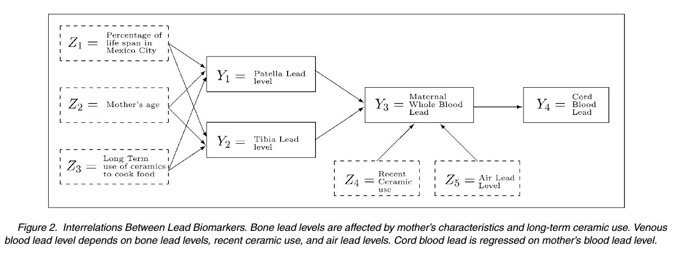
The first example is a model that explains the concentration of lead in four body tissues (umbilical cord blood, maternal whole blood, the patella, and the tibia tibia) via five environmental covariates (time living in Mexico City, age, use of ceramics for cooking [both long-term and recent], and the concentration of lead in the air). This isn't a case you'd normally think of as requiring the use of an SEM, but the model was structured hierarchically so that some of the response variables were also covariates for predicting the others. The figure below depicts the model's structure, with each arrow indicating a linear model. It was reproduced from the manuscript.

Since there are no latent variables in this model, we wondered whether the result of using an SEM to fit the data jointly will be very different from generating each regression model individually, and using its fitted values as inputs to the next level of the model.

The other example is a model for performance on eleven neurobehavioral tests with mercury exposure as an unobserved covariate that affects the latent factors "motor ability" and "verbal ability". Whale consumption was used to predict the mercury exposure (this study was conducted in the remote Faeroe Islands north of Scotland), with hair and blood mercury used as surrogates that reflect the mercury exposure. The diagram of this model's structure is reproduced below. Note that the double-ended arrow between motor ability and verbal ability indicates that the two latent factors are correlated.

One thing to note from the diagrams is that these models use a lot of parameters and impose a quite specific structure, both of which can be problematic. The number of parameters leads to concerns about the identifiability of SEMs, which must be carefully checked in each case, and the results may be sensitive to the structure, which must be chosen a priori, using the theory of the scientific field being studied. Model checking is discussed in the paper, but in a general way (necessarily, given that this is a review paper).

Both examples use linear models and Gaussian distributions at every stage, though SEMs can be used with more flexible model equations such as GLMs. The R package sem and the STATA package gllamm are called out as the state of the art (circa 2005).

We got to discussing when an Ecostatistician might want to use an SEM in their work, and the discussion focused around our favorite application: multivariate abundance modeling (mvabund). In fact, most kinds of regression and latent variable models seem to be specific cases of structural equation models (though that's not usually the most productive way to think). 

In sum, we found this paper to be a well-calibrated review article for statisticians who are looking to quickly understand the SEM methodology and see how it can be used in an example.

Paper of the year 2015

So we got together recently to discuss the papers we most enjoyed in 2015, and to vote one of them the Ecostats Paper of the Year. Top prize (nominator exempt from buying the next round of coffees or beers) went to James Thorsen's spatial factor analysis paper:

• Spatial factor analysis: a new tool for estimating joint species distributions and correlations in species range by James Thorsen et al., Methods in Ecology and Evolution, June 2015.

Joint species distribution models fulfil a need for ecological models that describe how species distributions are simultaneously affected by habitat and communities. Thorsen et al. combined spatial models with latent factors, and applied it to the US Breeding Bird Survey and to a dataset consisting of trawler transects for rockfish along the west coast of the US.

Other nominees were:

• A unifying model for capture-recapture and distance sampling surveys of wildlife populations by David Borchers et al., JASA, March 2015.

Capture-recapture and distance sampling are both common approaches to estimating the size of a population under study. Borchers et al. have developed a statistical framework which unifies the two, by introducing a spectrum for the spatial precision of individual observations.

• Model-based approaches to unconstrained ordination by Francis Hui et al., in Methods in Ecology and Evolution, April 2015.

Unconstrained ordination methods are widely used in exploratory analysis to identify similar and dissimilar habitats, communities, or study sites. By developing a model-based framework for ordination, Hui allows ordination to be used for statistical inference rather than purely descriptive uses.

• A guide to Bayesian model selection for ecologists by Mevin Hooten and Tom Hobbs in Ecological Monographs, February 2015.

 A very nice survey of Bayesian model selection methods from an ecological perspective.

•  A spatio-temporal point process model for ambulance demand by Zhengyi Zhou et al. in JASA, 2015.

This paper was noted as an excellent example of clear exposition and an unexpected application of point process modeling.

• Bayesian function-on-function regression for multilevel functional data by Mark Meyer et al. in Biometrics, September 2015.

Nominated as a change of pace that is likely outside the comfort zone of statistician used to analyzing typical ecological data, Meyer et al. describe a procedure for analysis of data that consist entirely of functional objects.

• Estimation and accuracy after model selection by Brad Efron in JASA, September 2014.

Efron's paper snuck in even though it was published in 2014. Model selection procedures like the LASSO are extremely popular among statisticians and ecologists alike, but the classical likelihood-based standard errors often don't apply post-model-selection. This paper proposes a general resampling-based theory of standard error estimation after model selection.

Analysis of ordinal data in ecology

The September Eco-Stats Lab (Friday 25th, 2pm, Bioscience level 6) will be on ordinal data analysis in ecology.

Ordered categorical data are commonplace in ecology when quantitative measurement of a variable of interest is not feasible or too costly. Examples include size of individuals, body condition and relative abundances of species. Cumulative link models are a powerful class of models for analyzing such data since observations are treated as categorical, the ordered nature is exploited and the flexible regression framework allows in-depth analyses.We will use the ordinal package in R to analyse some ecological ordinal data.

The code and details can be found here.

Welcome to Loic and Wesley!

We are very fortunate to have two new research associates joining us in Eco-Stats - Loic Thibaut and Wesley Brooks.

Loic came from a PhD at James Cook with Sean Connelly, and he will be thinking about how to resample generalised linear mixed models.

Wesley came here from Wisconsin, where he did a PhD with Jun Zhu, and he will be looking at the issue of spatial confounding and how it affects point process models.

Time to event analysis (Survival analysis) in ecology

The August Eco-Stats Lab (Friday 28th, 2pm, Bioscience level 6) will be on time to event analysis in ecology.

When modelling the time taken for an event to happen (e.g.death) we often use time to event analysis (survival analysis) rather than regression models. A common feature of these data is that for some subjects the even did not happen at all during the study period, called (right) censoring, and survival analysis can elegantly incorporate the information from these subjects. Regression models on the other hand have no easy way to include these subjects.

Survival analysis can often be applied to ecological data, e.g.

- Arrival of a parasite

- Survival times for animals/plants 

- Germination timing

- Response to stimulus

- How long fruit remain on plants before they are eaten

We will use the survival package in R to analyse some ecological time to event data.  You can find the code/explanation here, and the data here.